Early stage: tuned kernels reach about 10 to 17% of PyTorch; GPU robot simulation runs up to 126x faster than one CPU thread
GPU Robot Lab
GPU kernels written from scratch and benchmarked against PyTorch, then used to speed up a simulated robot. This page explains the first kernel, a tiled matrix multiply, and shows what has been measured so far. Code on GitHub.
1. Why a GPU kernel works on tiles
Multiplying two matrices means every output number needs a whole row of A and a whole column of B. Read naively, the same numbers get fetched from slow memory over and over. A tiled kernel gives each GPU program one small block of the output, then walks along K loading one tile of A and one tile of B at a time, so each loaded number is reused for a whole block of results.
Reduction = 2 x BM x BN / (BM + BN). The real kernel uses 64 x 64 tiles, which gives 64x fewer reads. The same formula is checked by a test in the repo (tests/test_tiling.py).
2. In what order should tiles run?
The GPU runs many programs at once, and they share a cache. If the programs running together work on a compact block of output tiles, they need fewer different pieces of A and B, so more reads hit the cache. Version 2 of the kernel launches tiles in groups to do this. The grid below numbers the tiles in launch order, and the shaded ones are the first 16 programs, imagined to run at the same time.
Fewer is better. This illustrates the idea and the arithmetic (checked by tests in tests/test_tiling.py).
Does it help the real kernel? Measured: yes, a little
Same tile settings, only the launch order changes. Speed relative to the plain row-by-row order (group 1), median of 10 repeats on a Tesla T4.
The grouped order is about 4 to 14 percent faster, best at a group size of 4 or 8, and a group of 16 gives little or nothing.
3. What has been measured
Tesla T4 on free Google Colab, 2026-10-20, 16-bit numbers. Every version gives answers that match PyTorch. Four versions are compared: PyTorch, the first kernel, the first kernel with the best settings from a 135-setting sweep, and v2 (automatic tuning plus the grouped launch order).
Repeated 10 times, v2 is about 3.4 times faster than the first kernel at 2048 and 3.5 times at 4096 (2.4 times at 1024, where the first kernel with the best sweep settings is faster than v2). It is 13 to 19 percent faster than the first kernel with the best sweep settings. Our kernels repeat closely, but PyTorch's own speed varies by 8 to 44 percent on the shared GPU, so the percentage of PyTorch moves between runs (10 to 17 percent here). The table and chart show one run; compare versions within a run.
Why the first kernel was slow
The first kernel used 255 registers per thread, the maximum, and spilled 84 of them to slow memory. Smaller K-tiles needed fewer registers and spilled none.
| Setting (tile, warps) | Registers | Spills | GFLOPS at 2048 |
|---|---|---|---|
| 64x64x32, 4 warps (first kernel) | 255 | 84 | 979 |
| 64x64x32, 2 warps | 64 | 972 | 90 |
| 64x64x32, 8 warps | 188 | 0 | 2,528 |
| 64x64x16, 8 warps | 118 | 0 | 2,807 |
| 64x64x16, 4 warps (best) | 200 | 0 | 3,035 |
Registers and spills come from the compiler for each setting. Speeds come from the 135-setting sweep (torch.matmul ran at 18,505 GFLOPS in that run). The link between spills and speed is a strong pattern, not a controlled proof. Pipeline stages hardly mattered (3,045, 3,036 and 3,035 GFLOPS).
Why PyTorch is still faster
The compiled code of every kernel setting we tried contains zero tensor-core instructions. It does its arithmetic with ordinary fused multiply-adds. PyTorch instead runs one library kernel, turing_fp16_s1688gemm_fp16_128x128_ldg8_f2f_nn, which takes 0.946 ms per call at 2048 (about 18,200 GFLOPS).
| Setting (tile, warps) | tensor-core instructions | plain multiply-adds |
|---|---|---|
| 64x64x32, 4 warps | 0 | 1,024 |
| 64x64x16, 4 warps | 0 | 512 |
| 64x64x16, 8 warps | 0 | 256 |
| 128x64x16, 8 warps | 0 | 512 |
This is the most likely main reason for the 6 to 10 times gap, but it is not proven: the kernel was not forced onto the tensor cores to see the change. Why Triton 3.6 produced plain multiply-adds on this older T4 is unknown, and a newer GPU was not tested. The s1688 in PyTorch's kernel name refers to a tensor-core instruction shape; that was read from the name, not checked against NVIDIA's documentation.
4. A robot, simulated in parallel
The same idea of doing many things at once applies to robots. The pendulum below has a motor too weak to lift it, so it must swing back and forth to reach the top. A planner tries thousands of motor plans at the same time in a simulator, keeps the best, and repeats. The final plan is then replayed in a separate simulator as a check.
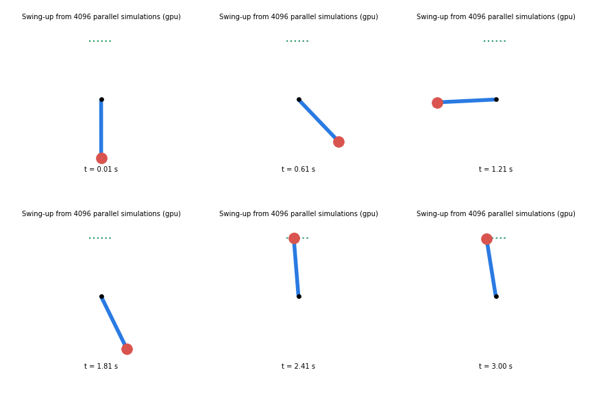
Planned on a Tesla T4 from 4,096 parallel simulations per iteration in 6.1 seconds (including compile time). Replayed in plain MuJoCo, the pole tip ended 0.494 m above the hinge, where the top is 0.5 m.
How much faster is the GPU?
Simulation steps per second for a pendulum, on a Tesla T4 (2026-10-20), median of 5 repeats, compared with one CPU thread (360,612 steps per second).
For a single robot the GPU is about 50 times slower than the CPU. It pulls ahead at around a hundred robots and reaches 126 times at 16,384. An earlier single run gave 129 times. Limits: a pendulum is very cheap to simulate, and the CPU baseline is one thread.
With collisions the picture changes
A box dropped on the floor (collisions and friction), same test. One CPU thread = 139,592 steps per second.
The GPU only breaks even at about 1,000 boxes and reaches 2.75 times at 4,096, compared with 82 times for the pendulum at the same count. When each step is more expensive, the GPU's advantage shrinks a lot, so the pendulum numbers are not typical for real robots. Larger batches were not tested, and this box is not a walking robot.
Is the planner itself faster on a GPU?
Seconds per planner iteration at the same batch size, compile time excluded.
Yes. The GPU is 2 to 26 times faster per iteration, and its time barely grows with the batch while the CPU's grows in proportion. Both found the same final heights. One run, against Colab's CPU.
5. A controller that learned
The swing-up above is a fixed plan. A better controller reacts to what it sees. Here a small neural network reads the pole's angle and speed and outputs the motor command. It was trained by trying thousands of slightly different networks at once in the simulator and keeping the ones that did best (evolution strategies).
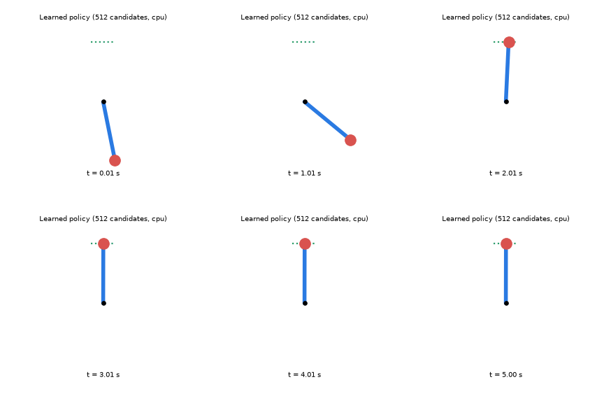
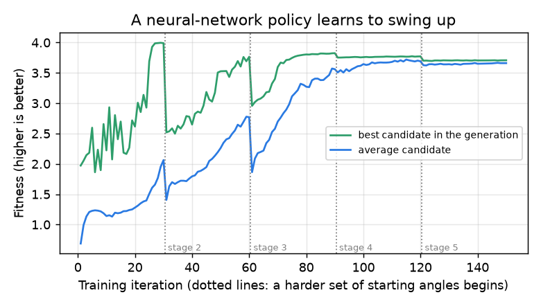
Trained on a laptop CPU in about 130 seconds with 512 candidates per iteration. Replayed in plain MuJoCo from five starting angles, including hanging straight down, it swung the pole up and held it every time, and the same happened with 3 different random seeds. But with more candidates it failed: a 2,048-candidate run on the CPU and a 4,096-candidate run on the GPU both ended with the pole rocking near the bottom, so the problem follows the population size, not the device. The cause is not found, and each larger size was run once. Two earlier versions also failed, and a five-stage curriculum, from nearly upright to hanging down, fixed the 512-candidate runs. One pendulum, evolution strategies, and the GIF is from a CPU run.
6. What is next
Find out which part of v2 helps (the tile settings or the grouped launch order) by changing one at a time, repeat the measurements to see how much they vary, and close more of the gap to PyTorch. Run the full experiment notebook on a GPU: which part of v2 helps, how much results vary, whether the kernel uses the tensor cores, whether the planner is faster on a GPU, speed with collisions, and the policy trained at a larger scale. Everything here runs on a free shared GPU. Run it yourself in Colab.